Wind-Aware Data Center Chiller Scheduling

FLIR thermal image of three chimneys in the wind tunnel at higher wind speed, with red lines tracing warm air from the first outlet over the downwind units. The scale runs from 23.4 to 72.9 degrees Celsius. — FLIR thermal image of the revised rig at higher wind speed, with a scale of 23.4 to 72.9 °C. The red lines are my traces of the plume.

The problem

A chiller's efficiency depends on the temperature of the air it pulls in. Downwind units breathe warmer air, so they need more power to deliver the same cooling. High-fidelity CFD can show this effect, but it is too slow to run every time the wind shifts, so the goal was a fast Python model an operator could use and understand.

Why the first apparatus changed

CAD model of the first test apparatus: blue chimneys standing in a round perforated plate on a foam base — The original rig: a 21-position laser-cut plywood grid, 7 in printed ABS chimneys and a wire-cut foam base.

Ansys airflow result around the round test plate, colored by vertical velocity — My Ansys airflow analysis, used to size the rig. It estimated a layer of about 1 in, for a 3 to 12 mph design range. The CAD and fabrication were shared with my teammates.

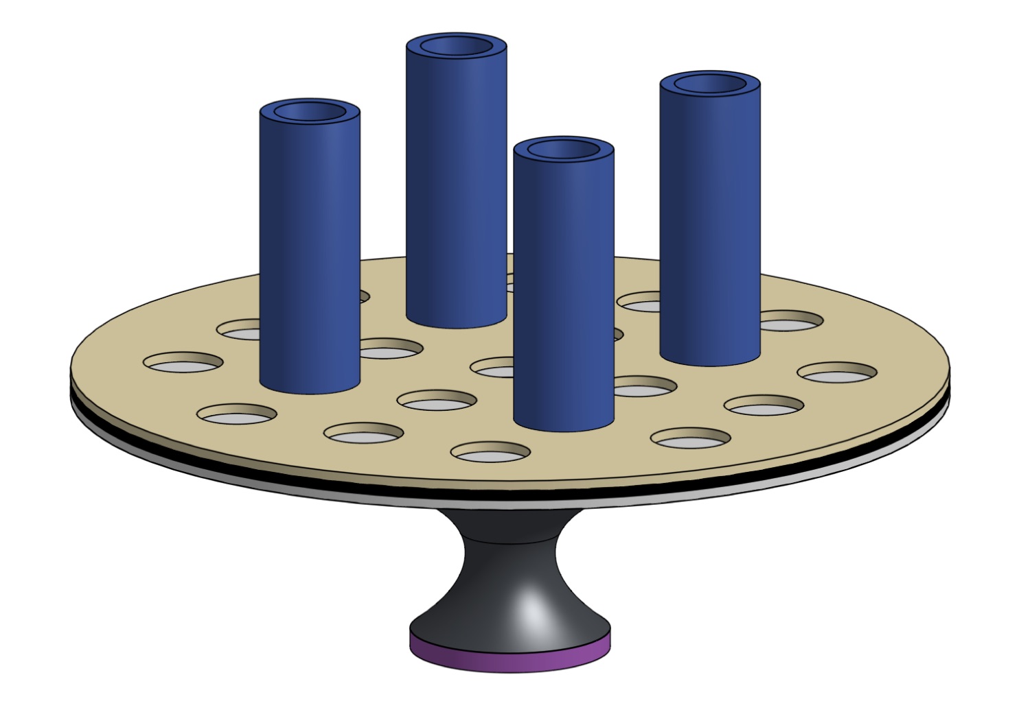
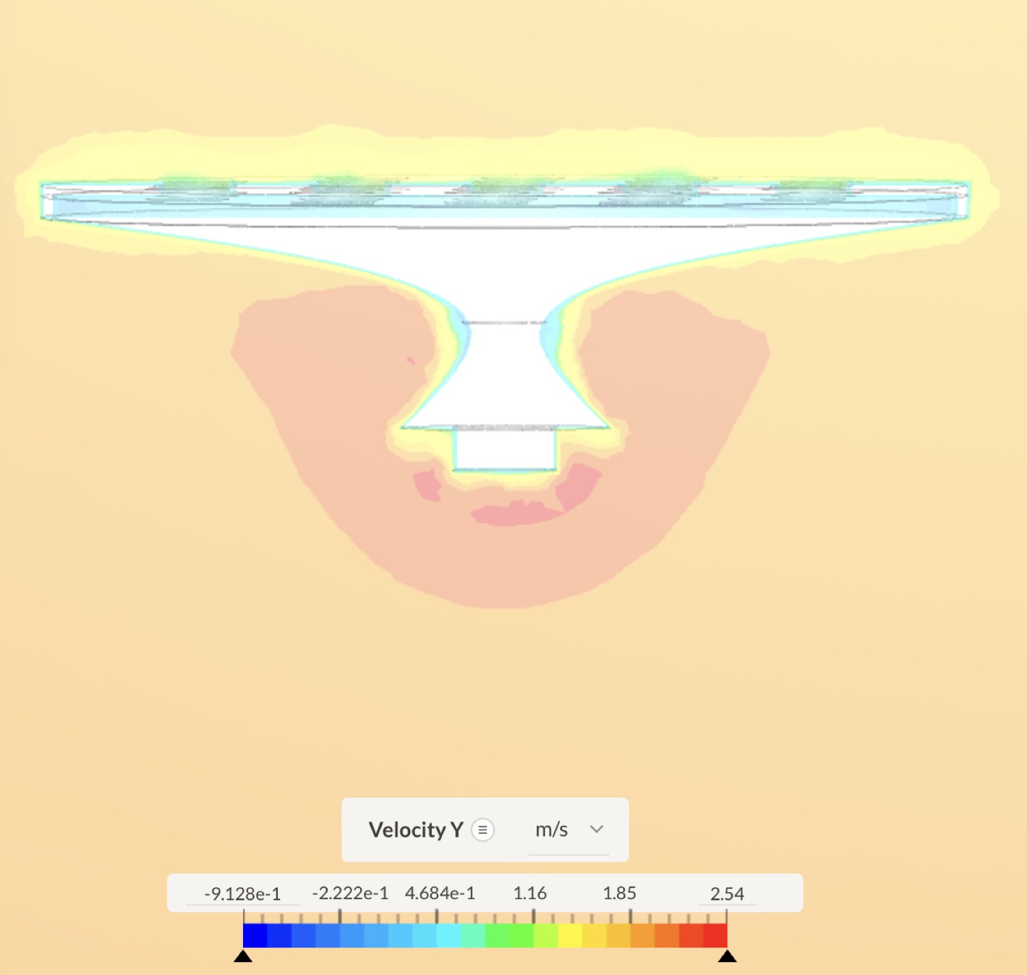
Intended measurement: See how each chimney's plume travels between units in a modular grid.
Observed problem: The candles used as a heat source kept going out, and the plume was hard to see when they stayed lit. Shielding, height changes and wind adjustments didn't make the observations reliable. The three-dimensional grid also limited the camera's view.
Change made: I proposed replacing the candles with the lab's smoke generator and moving three outlets into one row. A shared chamber feeds them, with an internal baffle meant to spread the generator's concentrated jet.
What it enabled: A camera could watch the source and the downstream plume from the side, and the rig produced usable visible and thermal records.

Design the experiment around the measurement you need.

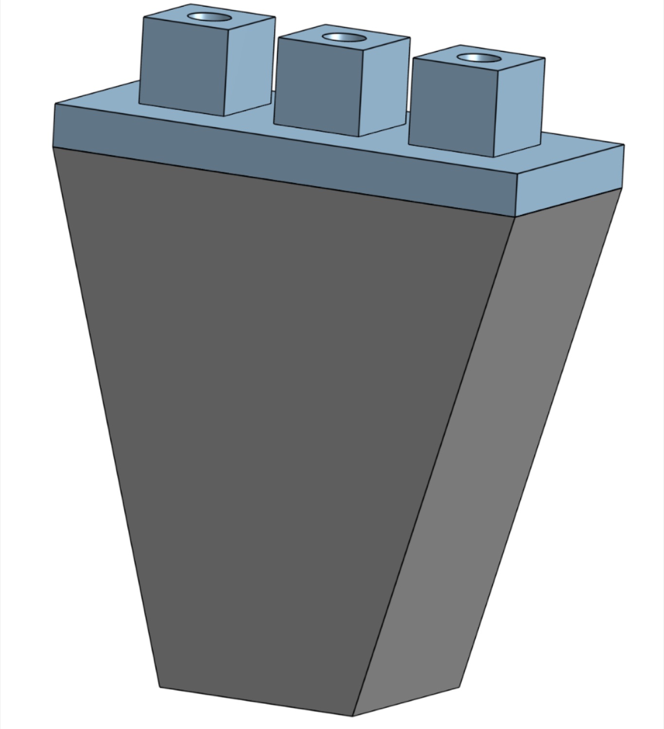
CAD model of the revised rig: three small chimneys in a row on top of a tapered chamber — The revised rig. I proposed the smoke source and inline layout, and laser-cut and assembled parts. The CAD was shared.

I helped define the revised dimensions, then laser-cut and assembled parts myself. My teammates shared the CAD and fabrication.

Two kinds of evidence

Physical observations from the rig and energy predictions from the model answer different questions, so they're kept apart here.

Source	Conclusion	Supported by
Rig observation	More wind made the visible plume more horizontal.	Lower-wind and higher-wind smoke images
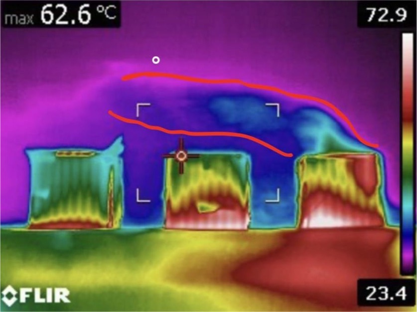
Rig observation	At high wind with all three outlets running, the downwind units sat in a warm dome and the last unit barely vented.	Smoke and FLIR images
Simulation	14.8% lower simulated energy use in one 24-hour scenario, against all units running.	Dashboard results
Simulation	That schedule used only some of the units, so it doesn't show balanced runtime.	Chiller utilization

What the experiment showed

This section is about plume behavior. The rig is a small smoke and thermal surrogate, and it did not measure chiller energy.

Smoke rising from three cardboard chimneys in the wind tunnel, with red lines tracing the edges of the plume — With the smoke generator running, the plume was clearly visible. I coordinated the tunnel testing and collected these images.

Cardboard chimneys in the wind tunnel at lower wind speed, with steep red lines tracing the plumes — Lower wind. The red lines are my traces of the smoke.

The same rig at higher wind speed, with flatter red lines tracing the plumes — Higher wind. The plume lays over. This pair is the visible evidence for the wind-speed observation.

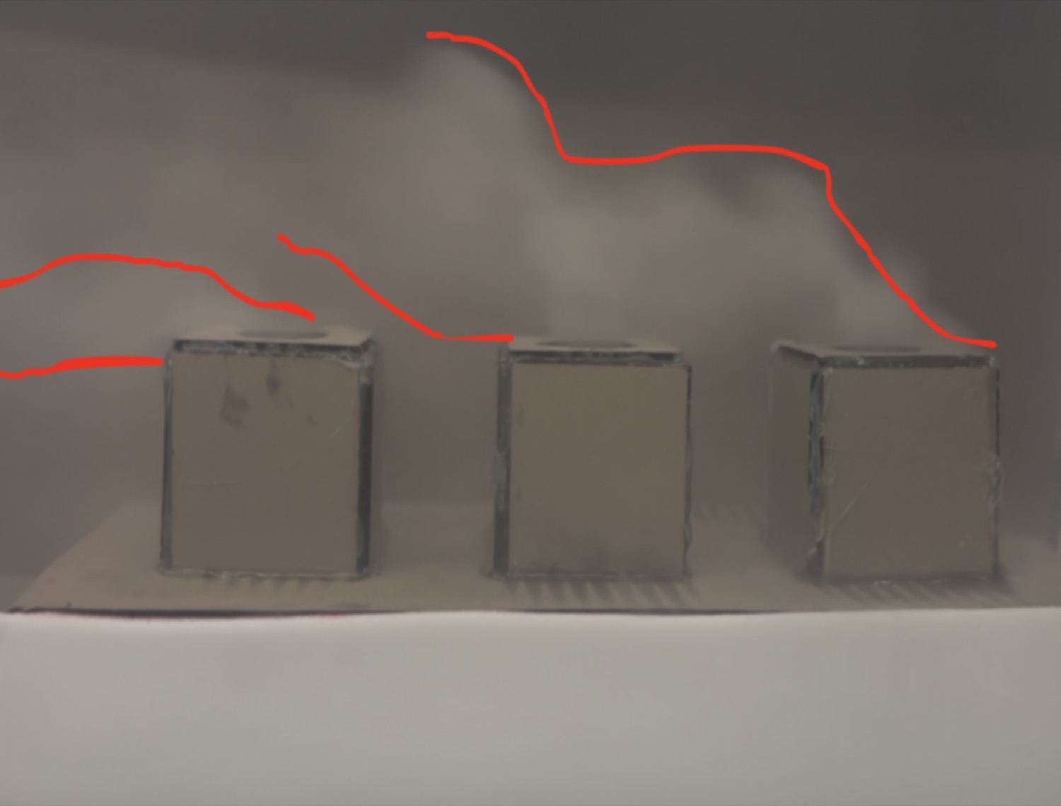
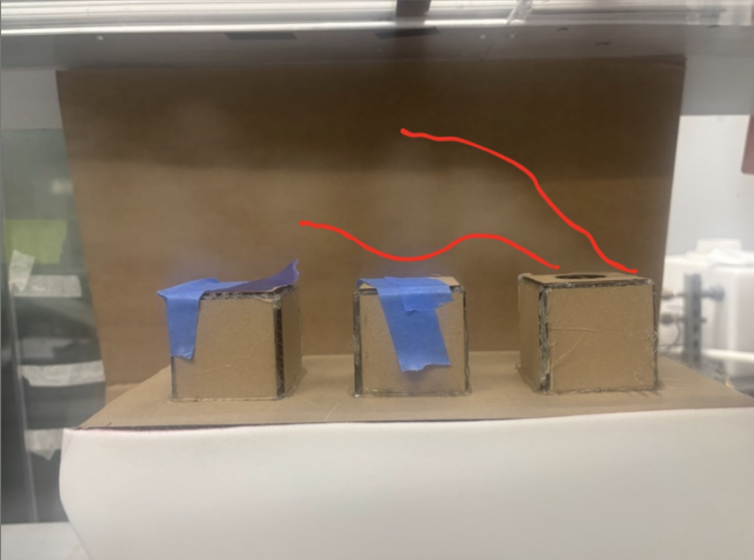
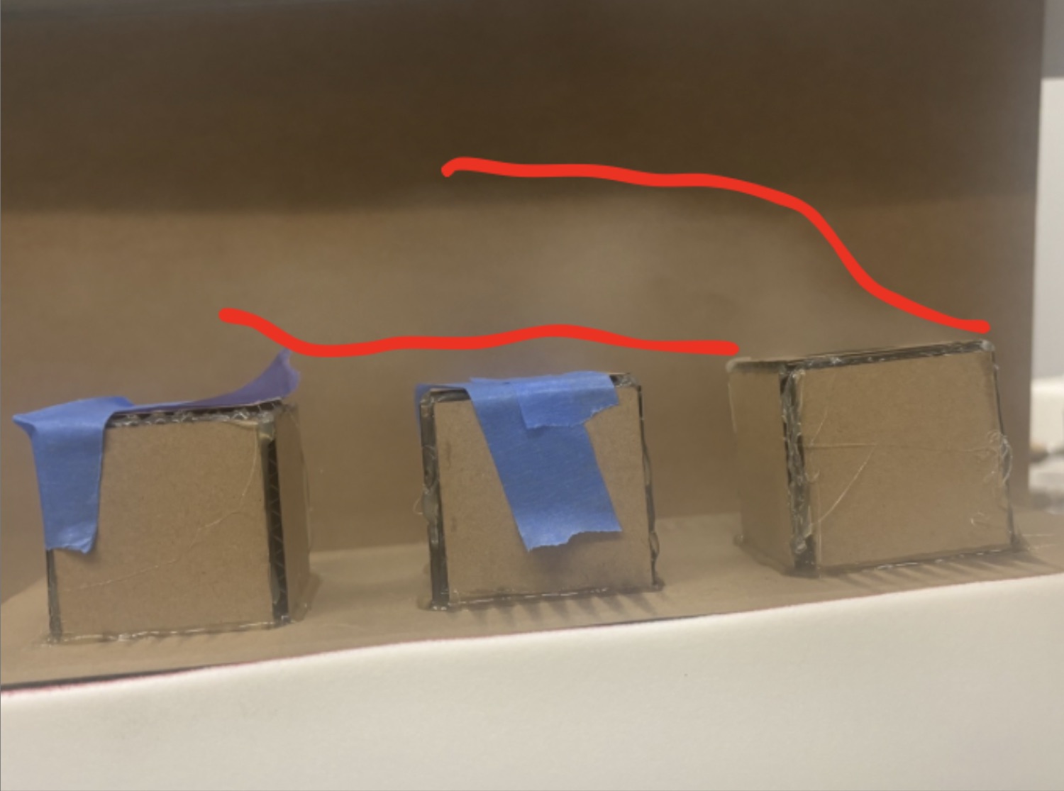
We ran three freestream speeds. More wind made the visible plume more horizontal, which is the behavior that can heat a downwind unit.

At the lowest speed the plume rose above the next unit, so its exhaust may never reach that intake. At the middle speed it leaned back into a dome of warm air over the downwind units, which is the shape our Gaussian model assumes. At the highest speed the dome got flatter and hotter.

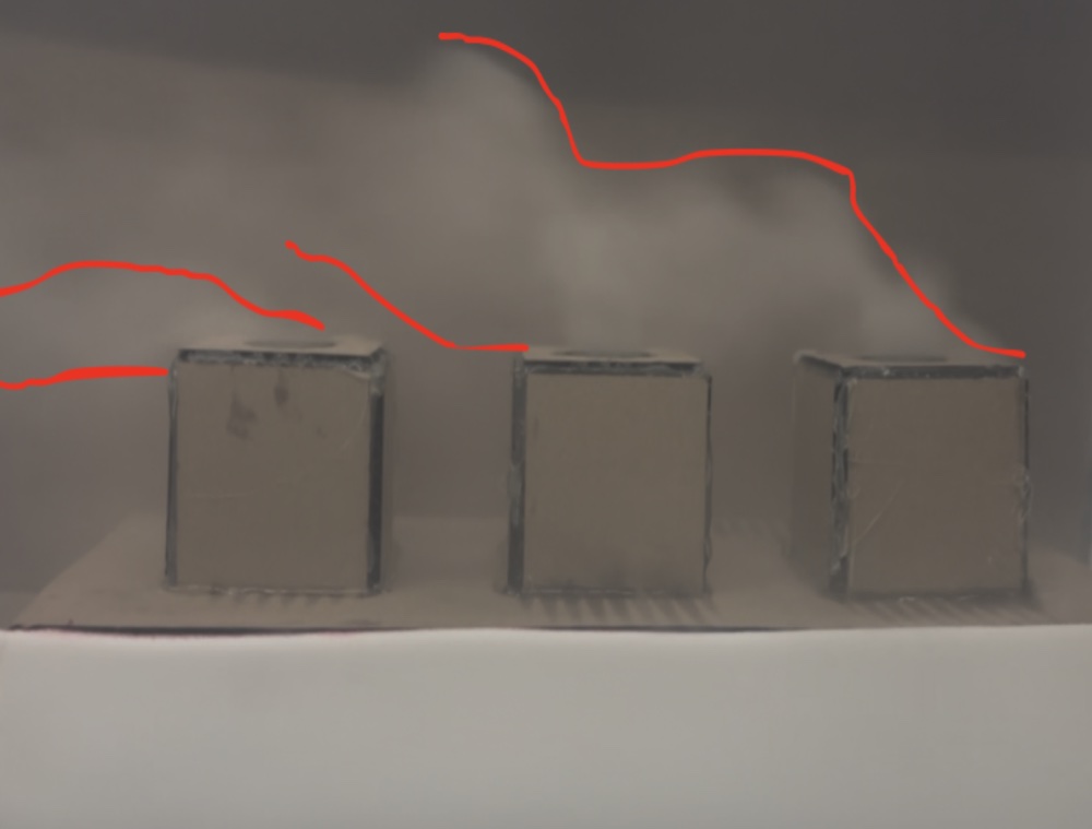
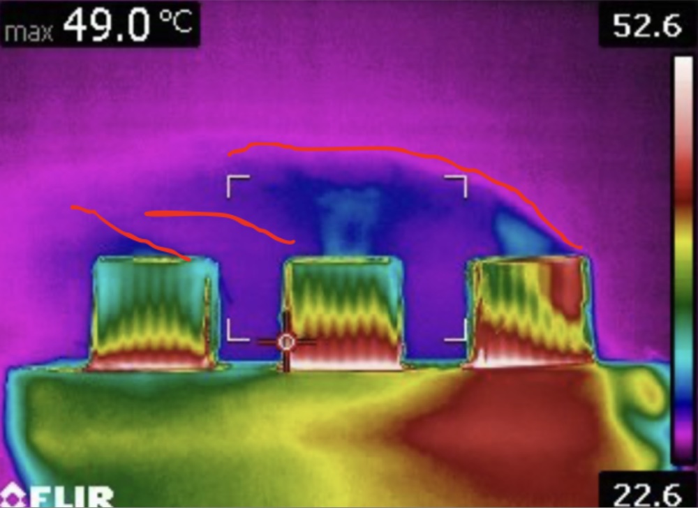
Three cardboard chimneys in the wind tunnel with smoke leaving all three, and red lines tracing the plumes — All three outlets running at high wind. The last unit vents very little.

FLIR thermal image of the same three chimneys, with a dome of warm air traced in red over the downwind units — The same case in thermal. The downwind units sit inside the warm dome.

We ran all three outlets at high wind as a worst case, since the exhaust has the least time to rise clear. The last unit barely vented, which we didn't expect. Our explanation, which we did not measure, is that the air slows as it passes each unit, leaving less fast, low-pressure flow to pull exhaust out of the ones downwind.

What the scheduling simulation predicted

This section is a model prediction. The wind-tunnel tests informed the plume model, but they did not validate the energy savings.

How the model works

Wind direction sets how far apart two units are, both downstream and sideways. A Gaussian term then estimates how much of one unit's exhaust reaches another, so a chiller's intake temperature is the ambient temperature plus a contribution from every active unit upwind:

T_in,m = T_a + Σ_k s_k A_km

That intake heating lowers the chiller's coefficient of performance, and the lower COP sets the power it needs:

COP_m = COP_0,m / (1 + α ΔT_m)
P = Σ_m Q_e,m / COP_m

A greedy search switches individual units on and off to reduce total power while still meeting the cooling demand.

The model runs behind a browser dashboard, where an operator sets the array, wind, temperature and load and then plays back the schedule. It only makes recommendations and doesn't control any equipment.

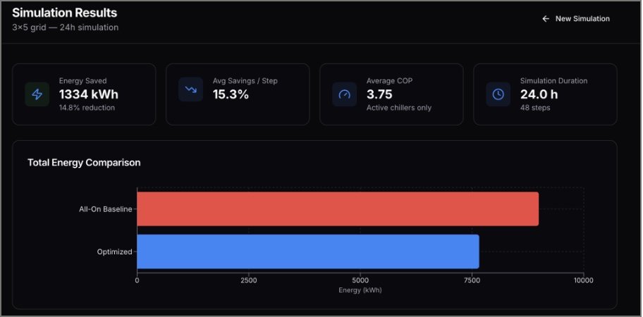
Dark dashboard panel titled Simulation Results for a 3 by 5 grid over 24 hours, showing 1334 kWh saved, a 14.8% reduction and an average COP of 3.75, above a bar chart comparing the all-on baseline with the optimized schedule — Dashboard output for the scenario. 14.8% is the reduction in total energy, the figure quoted on this page. The 15.3% tile is a different quantity: the average of the savings percentage across the 48 time steps. The modeling and scheduling work was shared, and Christian led the interface.

14.8% lower simulated energy use. In one illustrative 24-hour scenario for a 3 × 5 chiller array, compared with running every unit continuously. The energy comparison is a simulation result, not a measured reduction from an operating data center.

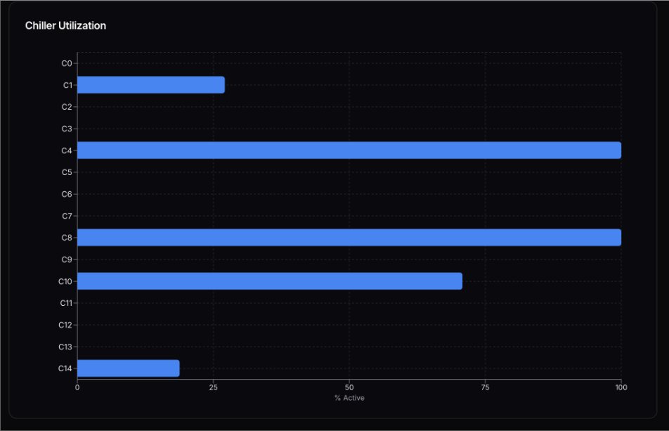
Bar chart of chiller utilization for chillers C0 to C14: C4 and C8 run all of the time, C10 about 70 percent, C1 about 27 percent, C14 about 19 percent, and the other ten units not at all — Chiller utilization from the same results screen. Two units run all the time and ten don't run at all.

This result demonstrates the method for one scenario. The utilization chart shows that it doesn't meet Trane's runtime-balance goal. The next step would be measuring outlet flow and checking temperatures and COP against independent data.

Report excerpt: apparatus setup and the simulated scenario

“The 2-D model was constructed to simulate three interacting plumes under supervised wind tunnel conditions. There are 3 in-line chimneys that vent the steam of a smoke generator.”
“In the Duke University wind tunnel, only the leading chiller was left unplugged. Steam was injected into the base of the physical model with the smoke generator. The plume shape was analyzed at 3 different wind speeds. A FLIR thermal camera and an iPhone camera were used to capture the plume shape.”

Final Report: Optimal Scheduling of Data Center Chillers, April 2026, team report. The report doesn't state the three tunnel speeds.

Inputs from the configuration figure and results from the results figure in the team's final report. Their duration and step count match, though the report doesn't state outright that they are the same run.
Scenario item	Value
Array	3 × 5, 10 m spacing
Chillers	Base COP 4, 500 kW maximum cooling, α = 0.7, ages from random seed 42
Wind	5 m/s, rotating ±60° about 90° with a 12 h period
Ambient and load	25 °C; sinusoidal load, 1,200 ± 400 kW, 12 h period
Duration	24 h in 48 steps
Reference	All units running
Result	1,334 kWh saved, 14.8% of total energy; average COP 3.75

Team

This was a team of four, with Christian Carbeau, Avery Estopinal and Senou Kounouho. Senou, Christian and I worked on scheduling, and Christian led the web interface.