Supersonic flow over a multi-angle compression geometry
I modeled Mach 2.2 flow through a channel whose lower wall turns the flow through three compression ramps and then an expansion, to see how the shocks and expansion change Mach number and pressure.
- Problem
- Predict how three compression ramps and an expansion change a Mach 2.2 flow.
- My contribution
- I modeled the flow in ANSYS Fluent and solved the first shock by hand.
- Engineering decisions
- I used first-order upwind discretization for stable shock capturing, accepting more numerical smearing. I kept the analytical first-shock solution separate from the CFD result, because one isolated ramp can't validate a flow with several interacting features.
- Evidence
- The dimensioned geometry, solver settings, Mach and pressure contours, line plots and the oblique shock calculation.
- Outcome
- The simulated flow slows in steps through the ramps and accelerates through the expansion.
- Scope
- This is a qualitative result. There's no grid-convergence study, and first-order upwinding smears the shocks.
- M₂ ≈ 1.88
- Analytical first-shock prediction of Mach number. Not a CFD validation result.
- p₂/p₁ ≈ 1.63
- Analytical first-shock prediction of static pressure ratio. Not a CFD validation result.
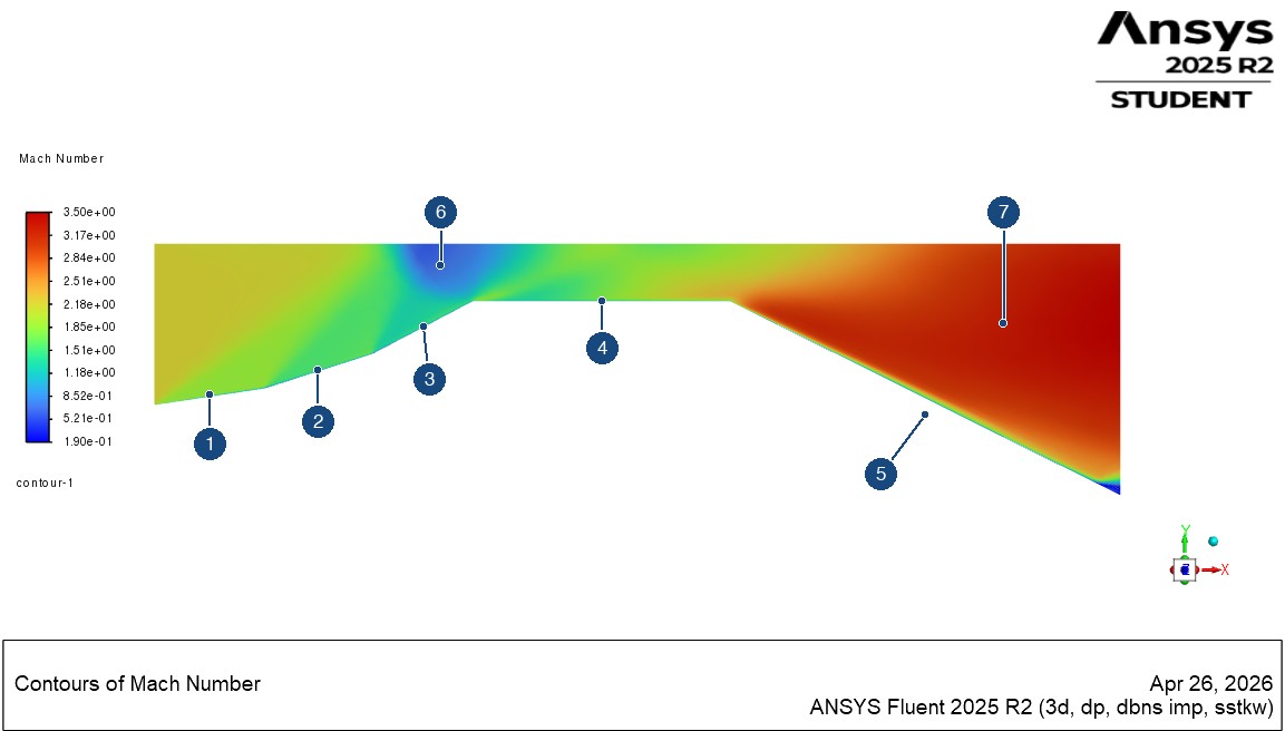
- 1: First ramp. A contour band starts at this ramp, the feature the analytical first-shock calculation addresses.
- 2: Second ramp. Mach number drops again as the wall turns further.
- 3: Third ramp, the steepest.
- 4: Flat section, below the region where the contour bands reach and cross.
- 5: Expansion. Mach number rises where the wall turns away.
- 6: Low-Mach pocket at the upper wall, above the end of the third ramp.
- 7: Highest-Mach region, downstream in the expansion. I didn't use it for a numerical check.
Geometry
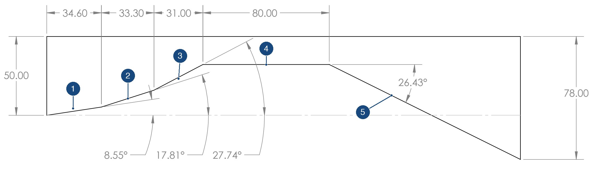
- 1: First ramp, 8.55°, starting at the inlet.
- 2: Second ramp, 17.81°.
- 3: Third ramp, 27.74°.
- 4: 80 mm flat section.
- 5: Expansion, where the wall drops away at 26.43°.
Solver setup
“Solver type: Density-based. Flow type: Steady, compressible. Energy equation: Enabled. Turbulence model: k-ω SST. Spatial discretization: First-order upwind for stable shock-capturing.”
“Inlet: Pressure far-field. Mach number: 2.2. Outlet: Pressure outlet. Walls: No-slip, adiabatic.”
“A structured mesh was generated with refinement near the geometry to capture shock structures.”
Analytical prediction of the first shock
I solved the first ramp by hand with the oblique shock relation, using M1 = 2.2, γ = 1.4 and θ = 8.55°:
tan θ = 2 cot β (M12 sin2 β − 1) / (M12 (γ + cos 2β) + 2)
The weak-shock solution is β ≈ 34.35°, which gives a normal Mach number of about 1.24. The normal shock relations then give M2 ≈ 1.88 and p2/p1 ≈ 1.63. These describe one isolated ramp, and the simulation includes the interaction of every feature.
Simulation results
The flow slows through the ramps, then speeds up sharply through the expansion. The strongest compression is at the upper wall above the end of the third ramp, where the contours show a pocket of low Mach number and the highest pressure in the domain.
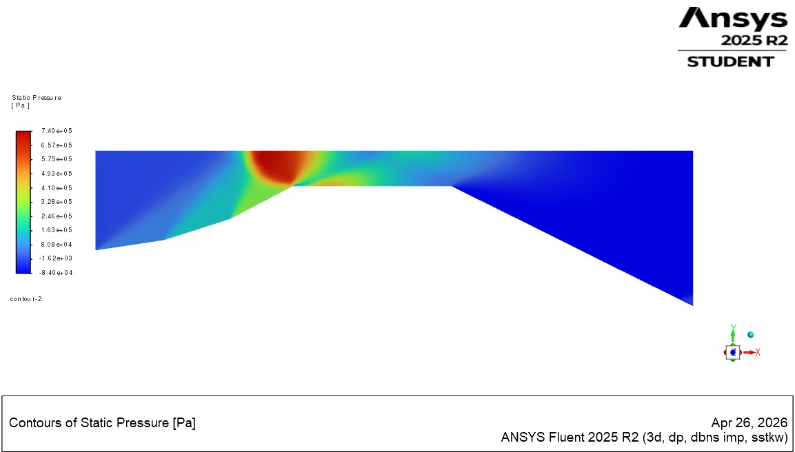
The two plots below sample the same Fluent line surface, labeled line-7, with a position axis running from about 0.01 to 0.075 m. The saved plots don't record the line's endpoints, so I can't say exactly where it sits in the channel or which shock it crosses at each point.
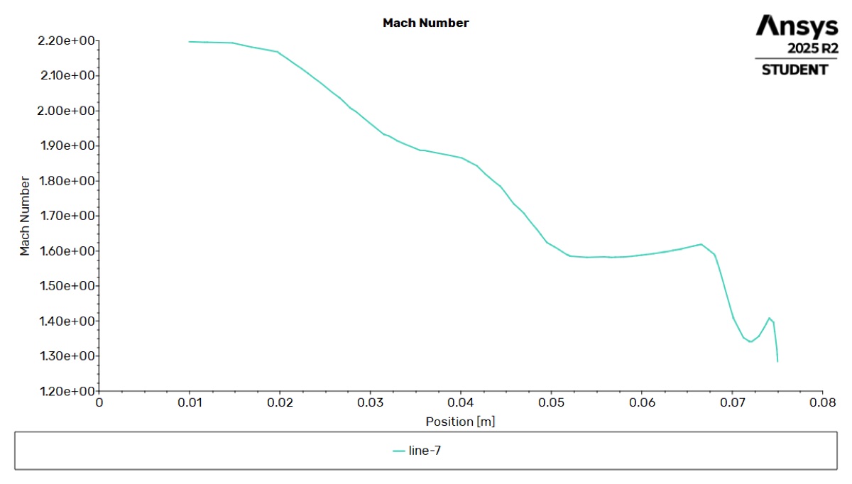
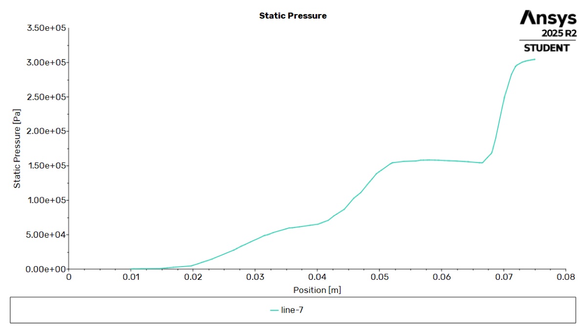
Mach number falls and pressure rises in steps along the line, which is the qualitative behavior compressible flow theory predicts. I'm not reporting a numerical comparison with the first-shock prediction, because the line's location wasn't recorded and the line data wasn't exported. The plotted pressures also can't be compared with the 1.63 ratio without the operating pressure from the case file, and reading values off the image would suggest more precision than it has.
Limitations
- First-order discretization. First-order upwinding adds numerical diffusion, which smears each shock across several cells and softens the steps in the line plots.
- No grid-convergence study. I didn't test how the results change with the mesh, so shock positions and contour values could shift on a finer grid and shouldn't be treated as precise.
- Comparison with theory. The hand calculation is a check on one isolated ramp. It doesn't validate the simulation as a whole.
Source file
- Supersonic duct: geometry drawing
One-page SOLIDWORKS drawing of the channel, with dimensions in millimeters.