PID control of a magnetic levitation system
An electromagnet can hold a steel ball in midair, but only with constant correction, because the system is unstable without feedback. My team built and tuned a PID controller in LabVIEW to levitate the ball and move it on command.
- Problem
- Stabilize an open-loop unstable ball and magnet, then hold a set height and follow changing position commands.
- My contribution
- I worked on the PID tuning and wrote the DAQ input and output in LabVIEW. All three of us brought up the hardware, built the PID VI and added the command modes.
- Engineering decisions
- We tuned one term at a time in height mode, stopping at Kp = 1, the highest value that kept levitation reliable. We then kept one set of gains for all four modes, so the controller was simpler to use and explain.
- Evidence
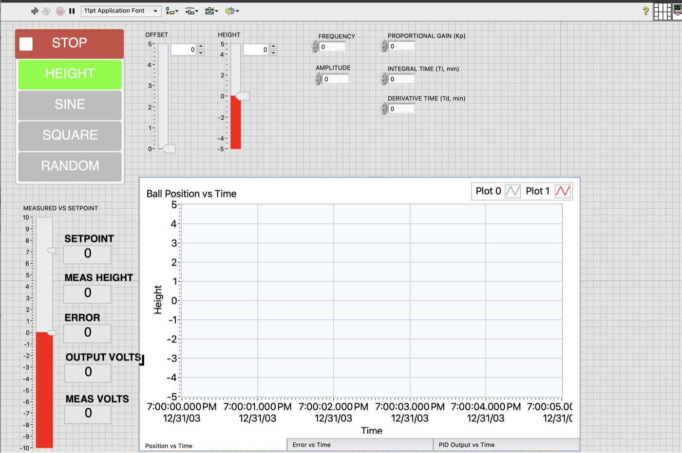
- A clip of the levitating ball, the LabVIEW block diagram and front panel, the calibration values and the tuned gains.
- Outcome
- The ball levitated and responded in all four modes with one set of gains.
- Scope
- These are observations from live charts during runs. Response traces weren't kept, so settling time and tracking error can't be reported from data.
- Kp = 1, Ti ≈ 3 s, Td ≈ 0.04 s
- Final gains, tuned experimentally and used for all four command modes.
The system in operation
The system
The rig pairs an electromagnet with an optical sensor that reads the ball's position as a voltage. That voltage goes through an NI DAQ board to LabVIEW, which sends a drive voltage back to the coil. Linearized around the operating point, the system has a pole in the right half-plane, so the ball falls or snaps to the magnet unless feedback catches it.
The model behind that statement
Gravity and magnetic force act on the ball, and the magnetic force grows as the ball gets closer to the magnet:
m ẍ = Fm − mg, Fm ≈ k i2 / x2
The linearized transfer function from control voltage to sensor voltage is:
G(s) = η / (s2 − ω02)
Calibration
We started by finding the operating point. The coil resistance of 22 Ω and a coil voltage of about 13.7 V, the midpoint of the manufacturer's 13.4 to 14 V range, give an equilibrium current near 0.62 A. My teammate AJ moved the ball through one ball diameter, 1.348 in, and recorded a 0.59 V change in sensor output, which gave a sensitivity of 0.438 V/in, or 17.2 V/m.
LabVIEW implementation
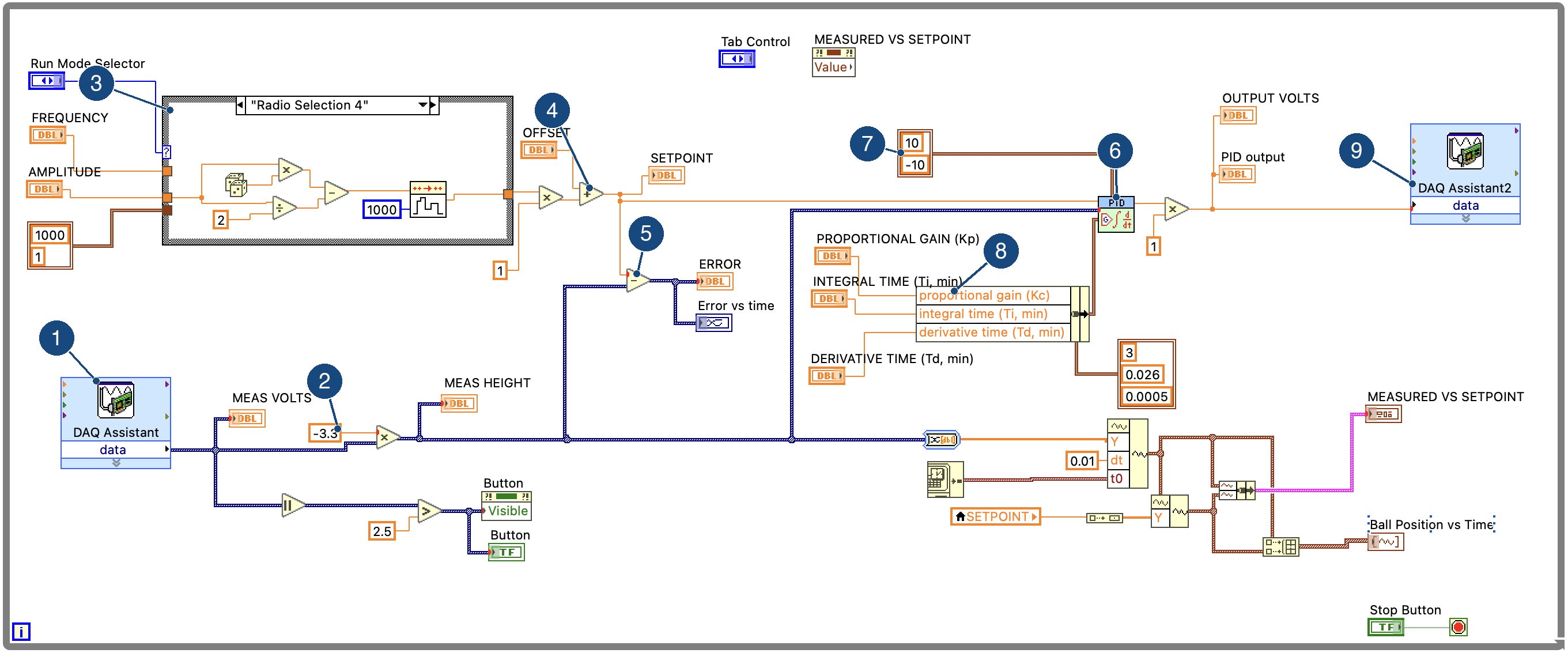
- 1: DAQ input. Reads the optical sensor voltage as MEAS VOLTS.
- 2: Voltage to height. MEAS VOLTS × −3.3 gives MEAS HEIGHT in display units. With 17.2 V/m, one unit is about 1.8 cm.
- 3: Command. The Run Mode Selector picks the case, using FREQUENCY and AMPLITUDE. The random case is showing.
- 4: Setpoint. The command plus OFFSET.
- 5: Error. Setpoint minus measured height, for the display and chart.
- 6: PID VI. Takes the setpoint and measured height directly.
- 7: Output limits. ±10 V, the range of the DAQ output.
- 8: Gains. The front-panel Kp, Ti and Td replace the default constants wired beside them.
- 9: DAQ output. PID output × 1 is written to the MagLev driver as the drive voltage.
Controller and tuning
We tuned the gains experimentally in height mode, one term at a time:
- Proportional. With integral and derivative action nearly off, we raised Kp until the ball hovered without oscillating wildly. Kp = 1 was the highest value that kept levitation reliable.
- Integral. Lowering Ti removed steady-state error, but values that were too small caused oscillation and overshoot. We settled on Ti = 0.0494 min, about 3 s.
- Derivative. A small Td of 6.87 × 10⁻⁴ min, about 0.04 s, smoothed the motion. Larger values amplified noise in the coil voltage.
We kept the same gains for every mode instead of retuning for each one, which made the controller simpler to use and explain.
What we observed
Height is a fixed-setpoint mode. Sine, square and random are changing-command modes.
- Height (fixed setpoint)
- The ball moved to the setpoint with a small overshoot. Settling took roughly 0.5 s, an observed estimate from the live chart and not a calculation from a saved trace. The output stayed inside the ±10 V DAQ limits.
- Sine (changing command)
- At about 1 Hz the ball followed smoothly, with some phase lag and slightly reduced amplitude. Both got worse as frequency increased.
- Square (changing command)
- Each step overshot more than the other modes, but the error returned close to zero before the next step. Early tuning reacted too aggressively to the steps until we raised Ti and added a little Td.
- Random (changing command)
- The ball moved the right way after every random step, and we never dropped it during our runs in this mode.
With more time, we would collect more data to fit a better model, tune separate gains for each mode, and save each run automatically so that settling time and tracking error could be calculated.
Team
This was a team of three, with AJ Vecchione and Shreyas Karadi. AJ measured the sensor sensitivity. The report's activity log credits AJ and Shreyas with finalizing the tuning and the front-panel layout.